Image Classification: An Introduction to Artificial Intelligence

This blog post will go broadly through the process of training a machine learning model. At the end, you will have a fully functional classifier with many interesting functions that hopefully spark your curiosity in this field of computer science.

Getting Started With AI

Let's begin with the fundamentals: and to do that, it's important to acknowledge that the term "artificial intelligence" is a bad start. When thinking of common examples of AI, usually artifical neural networks are referenced — specifically those with multiple layers, known as deep neural networks.

All of these networks belong to a broader family of machine learning systems. The word "machine" refers to computers, but the key word here is "learning." What does it mean that a program learns? It means that through repetition, it finds a way of doing things better. How it finds a way, and what better means, differ from project to project.

Generally, creating a machine learning system involves simple steps. You start with data related to the problem you want to solve, then you design and build a model. The model will need a carefully chosen measure for success and a cost function that it will try to minimize. After that setup comes the fun part: you feed the model your chosen data multiple times and measure the results.

Introducing Core Concepts

To get started, you will build a multi-class image classifier on the Fashion MNIST dataset using a convolutional neural network (CNN) model. Before diving in, let's unpack what that means.

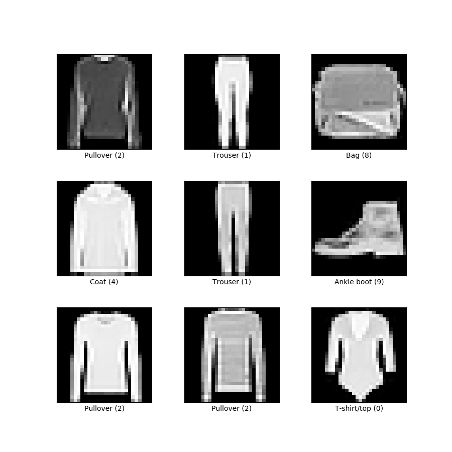
A classifier is a program whose objective is to tell whether an input belongs to bucket A, bucket B, or any other bucket. In this case the inputs are images, and the buckets are the classes: pullover, trouser, coat, bag, etc.

CNN refers to convolutional neural network (AI for the win!), which is an architecture of a neural network that has proven to be effective in processing images for machine learning.

The Fashion MNIST dataset is a commonly used benchmarking dataset composed of 28x28 grayscale clothing images that is available in Python's Keras library. MNIST stands for Modified National Institute of Standards and Technology.

Building An Image Classifier

Let's dive right into the code so that you can see the magic happening! I'll explain the most important aspects. You will be able to copy-paste this code as it is into Google Colab (or a Jupyter environment with the proper installations) and run it to see it happening live.

Step 0: Installing the right tools

This example builds the neural network with Keras, a Python lybrary that builds neural network models easily. a Python library that allows us to build Neural Network models easily. It was recently added to the Tensorflow package.

Jupyter Notebook cells execute Python code. When you want to execute system commands in them, use a leading !. This is one type of magic commands.

pip install -q -U tensorflow-addons

Then, import the building blocks for the Keras model: Matplotlib to visualize the learning progress, NumPy to do some data transformations, and Pickle to save our model.

These packages are installed by default in Google Colab. If you are not using that environment, you might need to install NumPy, Matplotlib, and Pickle using pip.

import tensorflow.keras as keras
from tensorflow.keras import models, Input
from tensorflow.keras import layers

import matplotlib.pyplot as plt
import numpy as np
import pickle

Step 1: Loading the dataset

Next, load the Fashion MNIST dataset. The collection includes 60,000 training samples, plus 10,000 testing samples. The X variables contain the images, and the Y variables contain their classes. They are arranged so that the first class in Y corresponds to the first image in X, and so on.

The test samples are meant to be used only once: at the end, when you will no longer make modifications to the model. At this stage in the learning process, you will use a subset of the train set.

(x_train, y_train), (x_test, y_test) = keras.datasets.fashion_mnist.load_data()
assert x_train.shape == (60000, 28, 28)
assert y_train.shape == (60000,)
assert x_test.shape == (10000, 28, 28)
assert y_test.shape == (10000,)

Step 2: Building the model

Now it's time to build the model. What does that mean? The model is just the architecture of the neural network: how many layers it will have, how many neurons per layer, how they are connected, and which functions dictate their learning behavior. This model is just a skeleton. It is empty and needs to be trained.

tf_model = keras.Sequential([
				layers.InputLayer(input_shape=(28, 28, 1)),
				layers.experimental.preprocessing.Rescaling(1./255),
				layers.Conv2D(16, (3, 3), activation='relu'),
				layers.Conv2D(64, (3, 3), activation='relu'),
				layers.MaxPooling2D((3, 3), strides=2),
				layers.Flatten(),
				layers.Dense(64, activation='relu'),
				layers.Dense(32, activation='relu'),
				layers.Dense(10, activation='softmax')
])

Let's go line by line into the most fun parts:

1. Sequential is a function that allows you to build a model through multiple layers. These layers are executed in order for every input.
2. InputLayer(input_shape=(28, 28, 1)) states that the shape of the input is a 28x28 matrix and has only 1 channel. The channel represents the color — in this case grayscale, and if the images were in RGB then this last number would have been 3.
3. Rescaling(1./255) will change the pixel integer values (which range from 0 to 255) into a floating point number from 0 to 1. Computers tend to think better this way.
4. Conv2D(16, (3, 3), activation='relu') creates the CNN part of the model. It will add 16 different filters of size 3x3 that will "convolute" over the image. The ReLU activation function is a very simple learning function that keeps positive values and transforms negative ones into zeroes. The next layer has 64 filters.
5. MaxPooling2D((3, 3), strides=2) is a convolutional layer with no training parameters. It will choose the highest value pixel in the 3x3 kernel, doing vertical and horizontal steps of 2 "pixels" each. (The details of Conv2D and MaxPooling2D will require another post)
6. Flatten() will transform the shape of the data from a matrix to a vector so that you can use "traditional" neural networks to finish its processing.
7. Dense(64, activation='relu') is a layer with 64 neurons, each of which is connected to every single neuron in the previous layer. The next layer has only 32 neurons.
8. The last layer, Dense(10, activation='softmax') has only 10 neurons, as that's how many different classes are in the dataset. The activation function Softmax assigns probabilities to every neuron so that they add up to 1. The chosen class of a given image will be the one with the highest probability score in this final layer.

Keras allows you to visualize the model by printing its summary:

print(tf_model.summary())

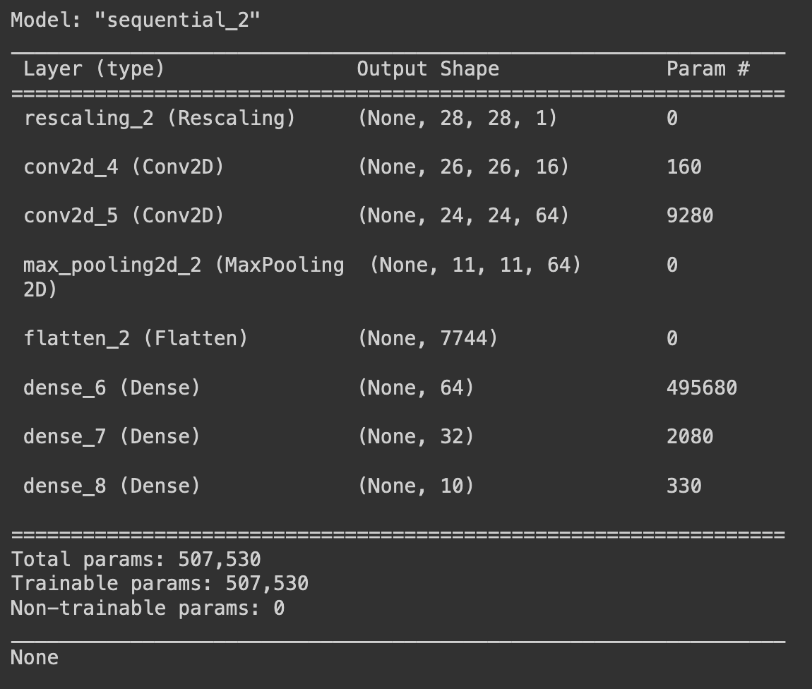
The layers of the model are arranged from top to bottom. Each layer is transforming the data into a different shape. The first layer has an output of the initial shape of the images, and the final layer has the shape of the number of different clases in the dataset. This model follows a pattern where the output shape of each layer first becomes bigger and bigger, until it starts decreasing gradually.

Step 3: Compiling and training the model

The cost function that the model will minimize is called a "loss function," and in this case you will use one called "sparse categorial crossentropy."

There are many different metrics you can use. This accuracy metric is not the best one for this problem, but it is easier to understand and research, so you'll use it in this example.

ADAM is a widely used optimization algorithm. For the purposes of this blog, you can think about it as a tool that will allow the network to learn better.

tf_model.compile(loss='sparse_categorial_crossentropy', 
																optimizer='adam', 
																metrics=['accuracy'])

Now you will use the dataset to train the model, but processing one sample at a time is too slow, so instead you will process them in groups, called batches. You will process the entire dataset 40 times to allow the model to learn through repetition, repeating each sample 40 times. One sweep over the entire dataset is called an epoch.

batch_size = 128
epochs = 40

Now execute the training part, which will take between 15-20 minutes to process.

fit_hist = tf_model.fit(
				x_train,
				y_train,
				batch_size=batch_size,
				epochs=epochs,
				validation_split=0.2
)

Note how you are not using x_test nor y_test anywhere. Instead, you are measuring the accuracy score of the model using 20 percent of the training set (validation_split=0.2), while training only with the other 80 percent.

This example uses an 80-20 split so that there are enough samples both in the training and testing split. However, depending on the size of a dataset, this could have been 75-25, 90-10, or any other useful ratio.

Every model has to be evaluated with data samples that were not used in the learning process so that you know how well it is generalizing the given patterns. If the score of the validation measurement was too low (e.g., 65 percent accuray), you would go back to change the architecture of the model and train again until reaching a desired validation score (e.g., 95 percent accuracy). That is a learning process in itself: If you used 100 percent of the train set and 100 percent of the test set, you would run out of data to evaluate how the model would behave with new samples once deployed in production. That is why you do not use the test set until the very end.

After iterating on the development of the model and reaching a useful validation score, one could then repeat the training with exactly the same conditions but now using 100 percent of the training set and evaluating with the test set.

Step 4: Plotting the training scores

After finishing training, you can visualize two scores: the training score and the validation score. You can see the training score by applying the metric to the samples that the model has learned from (80 percent of the training set), and you can find the validation score by applying the same metric to the samples the model has never seen (the other 20 percent).

plt.plot(np.arange(1, epochs+1), fit_hist.history['accuracy'], label='Train')
plt.plot(np.arange(1, epochs+1), fit_hist.history['val_accuracy'], label='Validation')
plt.title('Training accuracy')
plt.xlabel('Epoch')
plt.ylabel('Accuracy')
plt.legend(loc='lower right')

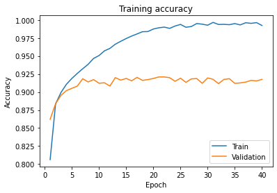
As you can see, the accuracy of the model improves as it processes the entire dataset multiple times. The Validation accuracy is more important to us, because it shows how well the model would behave if it saw new data. It improves steadily for the first epochs, but it reaches to a point where it stalls around 0.92. Meanwhile, the Training accuracy keeps improving. This means that the model is no longer generalizing, but is only learning the images of the dataset "by heart" (this is called overfitting). Your model will be able to learn from the dataset and is still able to manage data samples that it has never seen before.

If you sent a new image to this trained model, you would get a classification choice that would be 92 percent accurate. Cool!

Step 5: Saving our work

Once you've completed training once, you don't need to do it again. You can save the architecture and the values of the trained parameters in a file, and when you load it back up, it will function effectively the same.

# Save the model
tf_model.save('my_awesome_model.h5')

# Save the training history
with open('my_awesome_model_history', 'wb') as file_pi:
				pickle.dump(fit_hist.history, file_pi)

# Read the model
new_model = keras.models.load_model('my_awesome_model.h5')

# Read the training history
with open('my_awesome_model_history', 'rb') as file_pi:
				new_history = pickle.load(file_pi)

There are so many interesting topics to learn from this same program.

Recap

This post has gone through many concepts without going into detail. Machine learning is an exciting topic for me, and I hope you feel that it is at your reach too; you do not need a quantum computer nor magic to create a simple model. Broadly, machine learning models improve their goals through repetition, you provide an architecture and the data, and the program uses many standardized algorithms to arrive at a conclusion.

Did you notice how specific this project is? You built this model specifically to classify the Fashion MNIST dataset. It does not "know" that you can try to give it a picture of a cat. Nor will it try to build Skynet and conquer the world. Every project will be different, and different goals require different architectures and datasets.

Where To Go Next?

The code in this post has enough material for you to start asking many interesting questions and continue your learning journey. You can check out an example of this blog post [here](https://github.com/8thlight/ma...) Here are some of the ones that weren't answered in this post, that have very valuable knowledge behind them:

1. Why is the batch size 128, and why 40 epochs?
2. Can you further improve the 92 percent accuracy score?
3. Can you make the learning process faster?
4. Can you make the model smaller?
5. How can I avoid training from scratch if the training process is interrupted?
6. How do I modify one of my pictures into a 28x28 grayscale matrix to use in this model?
7. What exactly is a convolution?
8. What are ADAM, ReLU, and Softmax?

I hope you enjoyed building this simple image classifier, and that you store this model safely in your machine and happily in your heart. ❤