The first blog post in this series, "Image Classification: An Introduction to Artificial Intelligence," walks through the instructions on how to create a simple Convolutional Neural Network (CNN) for an image classification task. It did not explain the convolutional part of the network, and so it may remain odd why that machine learning architecture was appropriate. This post will show how machines can extract patterns from the data to solve image-related problems by leveraging multiple techniques and filters working together in a process called convolution.
Formally speaking, a convolution is the continuous sum (integral) of the product of two functions after one of them is reversed and shifted. It is much simpler in practice, and this post will use some basic examples that build up to it gradually. By the end of the post, readers should gain an understanding of convolution, familiarity with some of the image processing techniques that use them, and an awareness of how you might leverage convolution to solve image-related challenges in your own software development work.
Section 1: An Intuitive Convolution Example
Convolution is helpful for more than just image recognition, and its mechanics are easier to understand when applied to a more traditional challenge with numbers.
For this example, imagine a farmer who wants to have tomatoes available all year round. For that, they need to plant the tomatoes at different dates so they can be harvested at different dates too. How could one estimate the amount of water needed each month?
This array shows how many plants the farmer wants to plant in each of the following five months:
plant_batches = [1 2 3 4 5]
1 plant in the first month, 2 in the second, 3 in the third, and so on. So written as a function, it looks like: f(month) = plants. Over the next five months (array length), you will plant a total of 15 plants (array sum).
Now let's say that each plant will be ready to harvest in a single month, and it will take exactly 2 tons of water in that span. Calculating how much water the farmer will use each month is easy: just multiply each number of plants by 2 to get the answer:
water_per_plant = 2
total = [2 4 6 8 10]
You would need 2 tons of water the first month, 4 on the second, and so on.
Adding Another Variable
Let's complicate the problem a little bit. Let's say that each plant needs three months to grow (not one). And as they grow, they need more and more water to survive: 2 tons on the first month (month 0), 3 on the second, and another 4 in the third. This is now a second function with the form g(growth_month) = water_needed. So, if a plant is in its first month of growth, then you can calculate how much water it needs by calling g(0) = 2. This can be represented in the following array:
water_needed = [2 3 4]
Calculating how much water the plants need each month is now more complicated. On the first month, the farmer's first plant is in its first stage of watering. But on the second month, the first plant is in its second stage, and two newly planted tomato plants are in the first stage. Each of the five months initiates another round and layer of complexity, which can become overwhelming pretty quickly.
This is where a convolution is useful, and I'll walk through the steps for this example. First, flip the function (array) of watering stages. Then place both arrays side by side so that the first batch of plants is aligned with the first watering stage. Multiply the values that are aligned: 1*2=2.
 [1 2 3 4 5] // plant_batches
[4 3 2] // water_needed flipped
= 2

total = [2]
For the second month, move the watering stages one step to the right, multiply the aligned values (which are now two columns), and add their results. In this second month the farmer has one plant that grew and now needs three tons of water, and two new plants that each need two tons of water: (2*2)+(1*3)=7. The integration part comes by adding all multiplications.
 [1 2 3 4 5]
 [4 3 2]
= 7

total = [2 7]
For the third month, the farmer will have three overlapping columns:
 [1 2 3 4 5]
 [4 3 2]
= 16

total = [2 7 16]
Keep doing this until the last overlapping element, and you will end with a seven month watering plan. It will take seven months because the last batch that was planted in month five will continue to need water until month seven.
 [1 2 3 4 5]
 [4 3 2]
= 20

total = [2 7 16 25 34 31 20]
The watering stages array slid through the batches of plants. This is why you will find the sliding window operation continuously mentioned when referring to convolutions. This window (watering stages) is called the kernel.
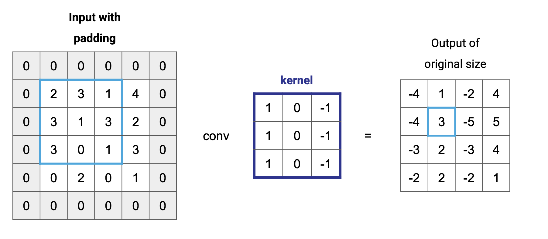
Section 2: 2-Dimensional Convolutions
The plant watering example is uni-dimensional, but the problem is similar with two dimensions. The window and the background will still be multiplied one element at a time, even when both of them contain two dimensions:
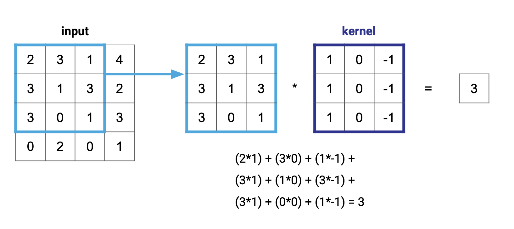
Performing a convolution on two dimensions just means sliding the window through every column of every row.
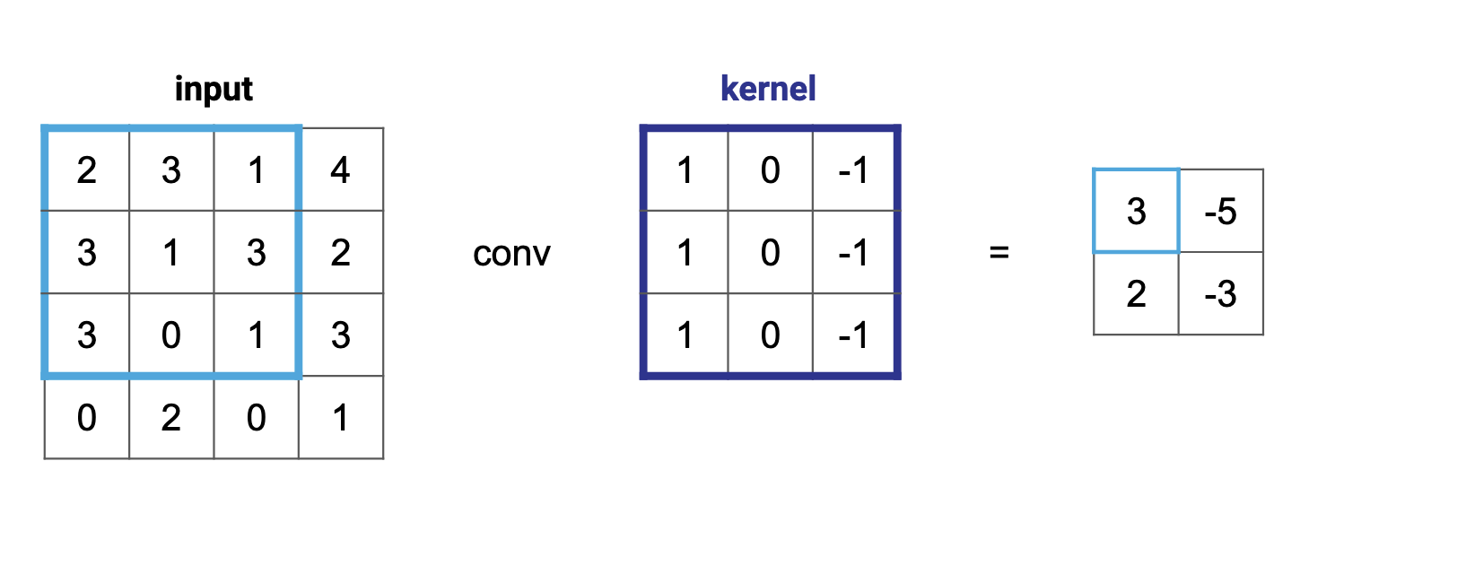
Notice how the kernel started completely inside the input background? This is standard for image processing, but there are other times (similar to the farmer example in Section 1) when you'll want to start the kernel outside of the input. In those cases, you can modify the output size by adding leading and trailing zeroes to the input. This is called padding, and it allows more multiplication operations to happen for the values in the borders, thus allowing their information to have a fair weight.
Section 3: Grayscale Images
Images are more involved than the simple examples in the previous sections, but they build on top of the same fundamentals. A black and white image is just a two-dimensional array with values that represent the intensity of each pixel. Higher values represent whiter shades, and lower values represent darker ones.
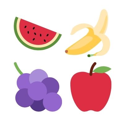
Let's take the following image as the input, and transform it into grayscale.
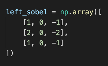
We can then apply a variety of different kernels to it, and print their results. For example, the following kernel is called left sobel:
If you convolve the grayscale fruits image with this kernel, and print the output as a grayscale image, it looks like this:
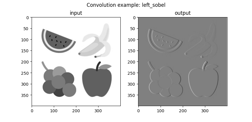
Why does the output look like it is casting a shadow to the right? The left sobel kernel has positive values in the left and negative values in the right. When the kernel is convolving over a homogeneous background, the multiplication of these values cancels out. However, when the kernel reaches the border of a fruit, one side of the kernel will produce a value that has more weight than the other (either positive or negative), and that difference will account for the new pixel's value.
When the contrast between the fruit and the background is larger, the kernel operation is larger too (positive or negative). That is why the apple, which has a larger contrast with the background, creates a border that is better defined than that of the banana.
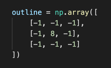
Another commonly used kernel is the outline:
Convolving the same grayscale image with it produces the following output:
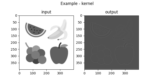
Can you deduct why the output looks like this? The kernel shows contrasting differences in a pixel and its surrounding elements, and as a result it creates both a dark and a light shade in each side of every border.
There are many more kernels that can convolute and generate interesting outputs for grayscale images. In the next section, I will go one step further and examine how a computer sees color.
Section 3: Color Images
The color on a computer screen is the result of mixing the three primary colors — red, green, and blue. Every pixel contains these three colors in varying degrees, resulting in the output appearing on a screen.
The important insight for this blog post is that a 2-dimensional image is actually a 3-dimensional array, as each color is given its own value at every coordinate: image[x][y] = [R, G, B]. Each channel (color) can be processed separately, and then joined back together to represent a color image.
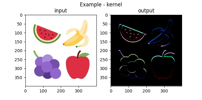
For example, using the left sobel kernel on every channel in the original image before combining yields this result:
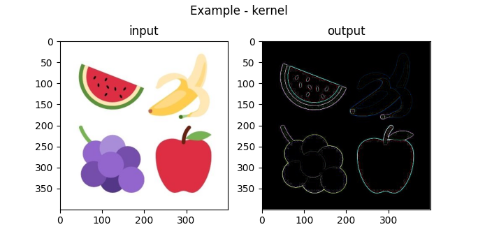
And using the outline kernel produces this result:
Using The Gaussian Kernel
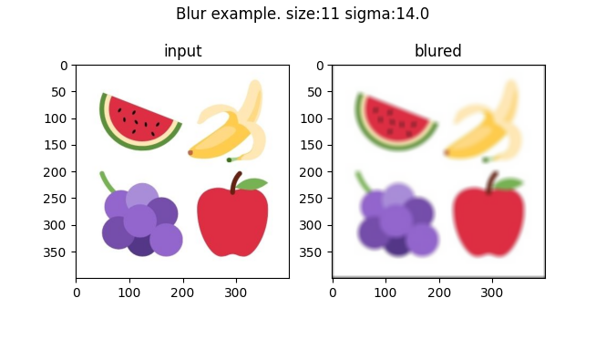
Another interesting kernel is a gaussian kernel. This function takes values of a gaussian (or normal) distribution and places them in a vector to compute the outer product with itself. For example, given 5 discrete values of the gaussian distribution, the outer product will be a (5, 5) matrix. The kernel then normalizes those values so that they add up to 1. This creates an average sum of pixels that gives more weight to those in the center of the kernel. Executing this convolution in each color of the input image produces a blur effect.
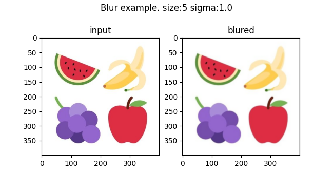
Increasing the kernel from (5, 5) to (11, 11) and with a higher standard deviation of the initial gaussian distribution yields a stronger blur:
Notice how the output is 3-dimensional (height, width, 3) despite using a 2-dimensional (11, 11) kernel. This is because this kernel has only two dimensions (x, y). If instead, you used a 3D kernel of shape (11, 11, 3), it would only slide in the x and y directions, so the output would be a 2-dimensional array. One would iterate this rectangular cuboid over the 3-dimensional RGB image to produce a 2-dimensional array.
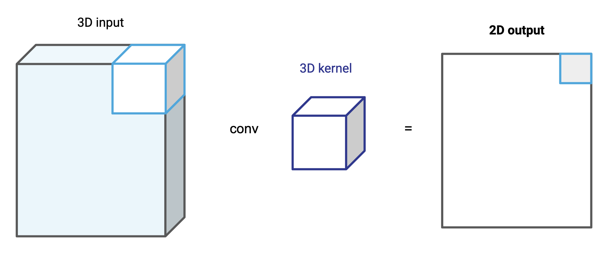
Computers do not need an input to have exactly three colors — they can have 10, 20, or as many channels as we want. As long as the kernel is exactly of the same depth, it will generate a 2-dimensional output.
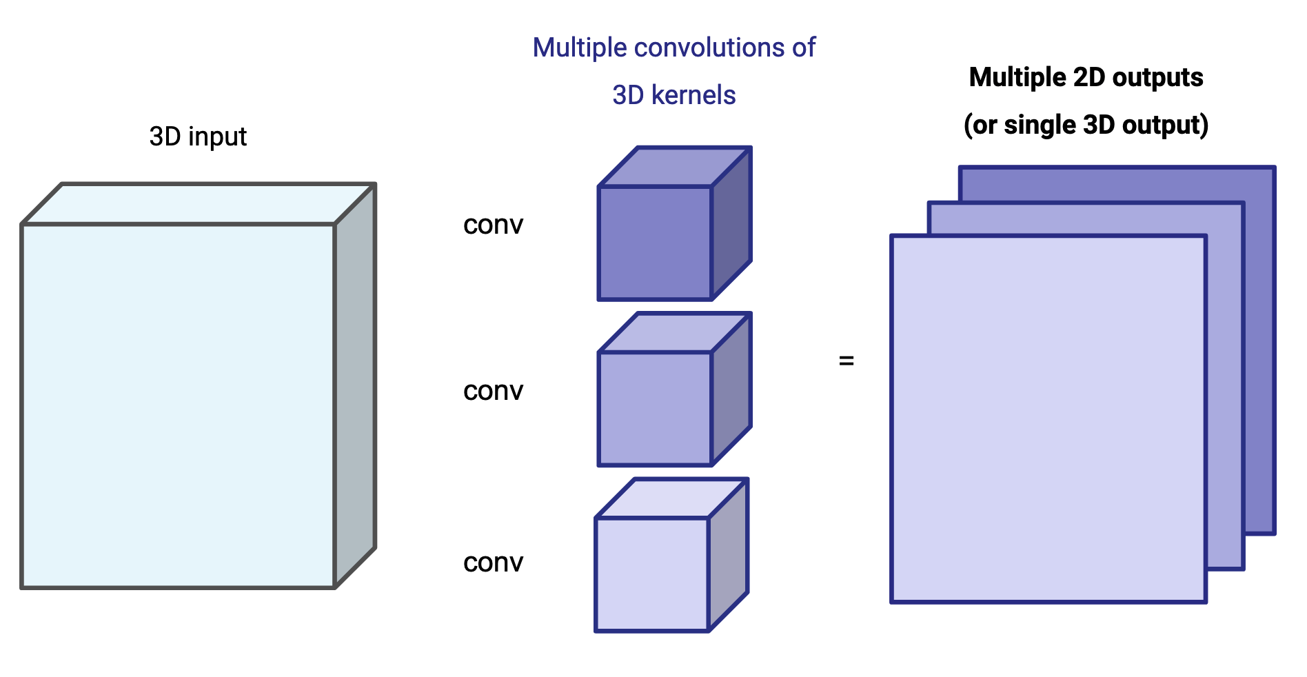
Now let's take it one step further: take two different 3D kernels and execute the convolution over the same input. This will result in two different 2D arrays, which can be portrayed as a 3D array of exactly two channels.
This opens up a world of possibilities. One can stack multiple convolutions using multiple kernels, creating a single output of an arbitrary depth (the number of kernels dictates the depth of the output). This output can be further convoluted again using the same logic, creating chains of convolutions that build on each other.
The problem is that infinite possibilities is too much for a human being; and that is where machine learning comes in.
Section 4: Relation To Machine Learning
Each kernel provides different information. In the grayscale fruits example, the left sobel kernel shows vertical borders and the outline kernel shows differences in contrast. These visual representations are patterns that humans can understand, but computers can create their own kernels based on patterns that only they can understand.
Convolutional Neural Networks (CNNs) are a common network architecture used for processing images for machine learning. CNNs change the values of the kernels when learning so that they are optimized for the task at hand.
Imagine that we want a machine learning model to learn 16 kernels of shape (3, 3, 1) (2D) and to convolute over the same input of size (28, 28, 1) (2D). The resulting output will have a depth of 16, one for each kernel.
In order to learn, each kernel needs an extra parameter called bias. Thus, all 16 kernels need to be trained for (3*3*1)+1 = 10 parameters, for a total of 16*10 = 160 parameters in each convolutional layer. This is exactly the number of parameters shown in the conv2d_4 (Conv2d) layer in the summary of the previous post:
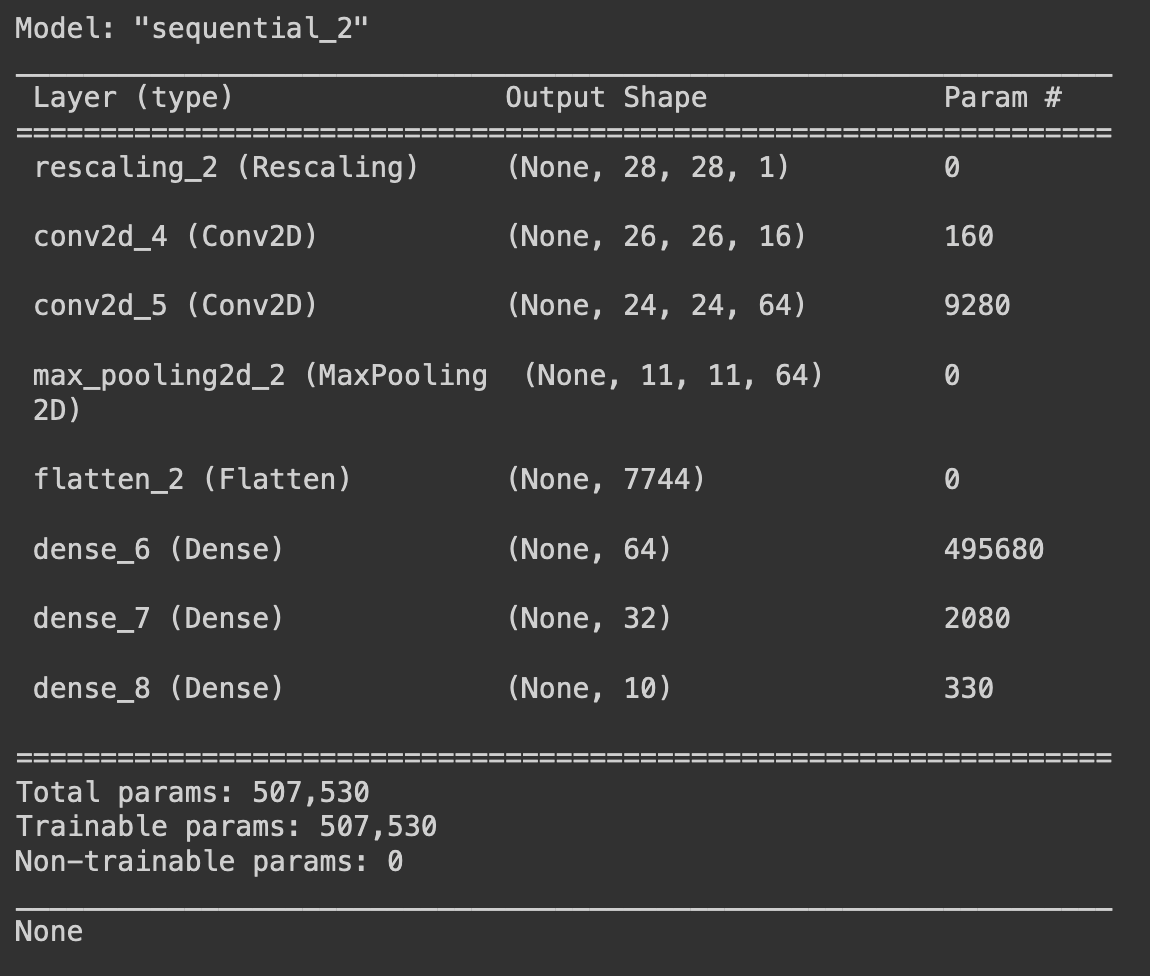
The next layer, conv2d_5 (Conv2d), is a bit trickier. Its input shape has a depth of 16 (one for each kernel in the previous layer!), which means that each 3x3 kernel is actually a cuboid of shape (3, 3, 16). Each of them then needs to learn (3*3*16)+1 = 145 parameters. Because there are 64 kernels, then the total training parameters for that layer is 145*64 = 9280. Don't worry too much about the bias parameter right now, what is important is understanding what a convolution means and what a machine model learns when using them in its layers.
What the model will learn for values in these kernels will make no sense for a human eye, especially the second layer. But we can still use it. The shape of the layer is further transformed into a single vector using Flatten. If the 2D output was of shape (11, 11, 64), then the size of the flattened vector will be 11*11*64 = 7744. This can be fed easily into a traditional dense layer.
So why bother going through the convolutional layers if we can flatten the images? Because the relationships between pixels are helpful clues. Pixels that are close to each other must share some information, and convolving over the entire image at the start might flatten these connections, filtering out abstractions through the layers and leaving the machine to learn through intense repetition alone.
Recap
This blog post explained what a convolution is, and some common image processing techniques that use them, like blur and some border recognition convolutions. It also touched the concept of padding and how it affects the size of the output. The examples went from a 1D convolution to a 3D convolution, and introduced the sliding-window operation.
Finally, the examples showed what is being learned in a convolutional neural network, and we were able to count the exact number of parameters for its layers. Hopefully you are able to see why using convolutional neural networks are useful for visual tasks like the image classification of the previous post.
Where To Go Next?
With this theoretical knowledge, you could start thinking of building a simple convolutional method and experiment with some interesting kernels. You can check out a python implementation of this blog post here. I recommend checking out other kernels, like the other three sobel kernels, the sharpen kernel, and different sizes of the gaussian blur. You can learn more about how the kernels interact by experimenting with, say, blurring an already blurred image over and over again, or applying one sobel after another.
With regards to neural networks, this blog showed how a convolutional layer is used to process an image. Can you imagine different approaches to process a video? Would you handle the time dimension with a 4D kernel, or would you process each frame separately using 3D kernels?
I also recommend checking out Python's OpenCV library for a vast collection of other image processing tools. One could imagine using a 1D kernel to process time sequences like stock prices and daily covid infections over a year.
Once you learn to harness your computer's processing power into machine learning tasks, your imagination is the limit.