


My first experience with SQL performance tuning came before I decided to pursue programming as a career.
As a Business Intelligence Manager, I was tasked with developing a method of predicting consumer purchasing trends and stocking the most commonly purchased items. This involved slow-plodding SQL queries over millions of rows of consumer purchasing data. Eventually, the slow feedback cycle became untenable.
I had a discussion with our database admin about optimizing the SQL queries, and it was quickly pointed out that I was heavily reliant on queries on non-indexed fields. We created a number of new indexes and, lo and behold, the queries completed in a flash.
From then on, I would proactively check the indexes as I was implementing new stored procedures, but I never quite knew what was happening under the hood.
Querying Without an Index
When a query is run on an SQL database, the database engine executes a search function. The simplest search to implement is a linear search. A linear search is like searching through a book for a desired page starting from the front of the book and checking every page number in sequence. It starts at the beginning and checks every value until the desired one is found or the end is reached.
If we look at the complexity of linear search, which would be a query on a column without an index, the Big O notation would be:
O(n)
As the number of records increase, the search time increases directly in relation to the number of records. A linear search which executes in 0.05 seconds would take 1000 times longer on a dataset 1000 times the size, around 50.0 seconds.
If the query is performed often on a non-indexed column, it is probable that creating an index will improve performance.
Default Indexes
Creating an index in a SQL database changes how the data is searched. In MySQL, PostgreSQL, and Microsoft SQL, the default index data structure is a B-Tree.
B-Tree based indexes are created by default on any primary key, foreign key, and uniquely constrained fields. While other indexing methods are shipped with the major SQL distributions, B-Tree is by far the most common and will be the focus of the remainder of this article.
Origins of the B-Tree
The B-Tree was created by Rudolf Bayer and Ed McCreight in 1971 while working at Boeing Research Labs. The name was crafted over lunch. Ed explains his naming decision best.
“Bayer and I were in a lunchtime where we get to think [of] a name. And … B is, you know … We were working for Boeing at the time, we couldn’t use the name without talking to lawyers. So, there is a B. [The B-tree] has to do with balance, another B. Bayer was the senior author, who [was] several years older than I am and had many more publications than I did. So there is another B. And so, at the lunch table we never did resolve whether there was one of those that made more sense than the rest. What really lives to say is: the more you think about what the B in B-trees means, the better you understand B-trees.” - Ed McCreight, 2013
B-Tree Complexity
A B-Tree is a tree data structure that self-balances and has a log(n) search complexity. This means that the search time through the tree is drastically reduced compared to a linear complexity search.
A B-Tree index consists of levels of pages (or index nodes) that make up the levels of the tree. The top node is the entry point into the index, which is also referred to as the root node.
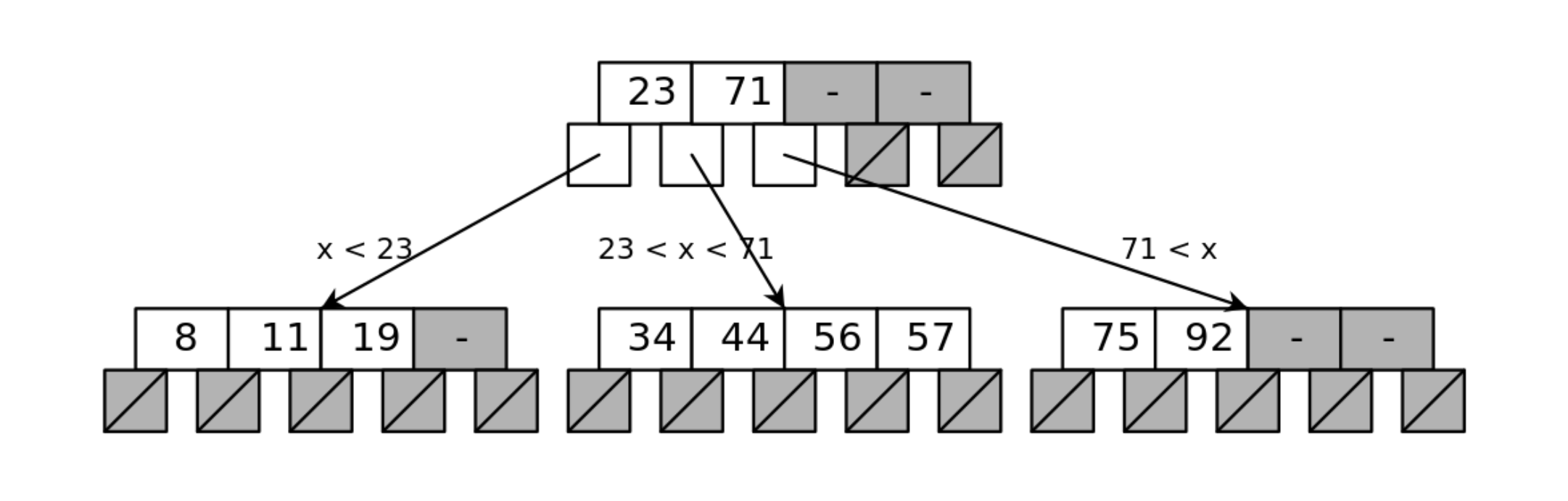
When creating an index, a specific column is chosen as the values to be indexed. Each node has a range of values representing the values from the column indexed, and is segmented to represent the ranges of values represented in the child nodes.
In the example above, the entire tree contains values from eight to 92. The root node has three child nodes, each of which represent a somewhat equivalent section of the indexed values at the level.
The root node contains two numbers which segment the data into the three sections. If the value requested is lower than the lowest value in the root node, the left child node is returned. If between the values, the center node is returned. And if greater than the highest value in the root node, the right child node is returned.
This same branching takes place at each level of a B-Tree, until the requested value is reached, or the value is found to not exist. Each index value contains the key to be matched, and a pointer to the record in the database table.

Searching Through a Book
Imagine a 100 page book which is segmented into four sections. It has nice blue tabs stuck to pages 25, 50, and 75. If the number we are searching for happens to be 25, 50, or 75, then our search ends at that page. If not, then we have four sections with which to look for the next page value. If our page is 24, we open the section before the first tab, if between 24 and 50, we open the second section and so on. This is a log search complexity. The linear search complexity would be to start at the front or back of the book and compare every page number to our desired page number.
While each node is searched in linear time, the tree branches in such a way that the data set is searched in log n time. Below is the Big-O notation for a B-Tree search.
O(log n)
A B-Tree search which executes in 0.05 seconds on a small dataset would scale much better than a linear search. Below are the search time comparisons for illustration.
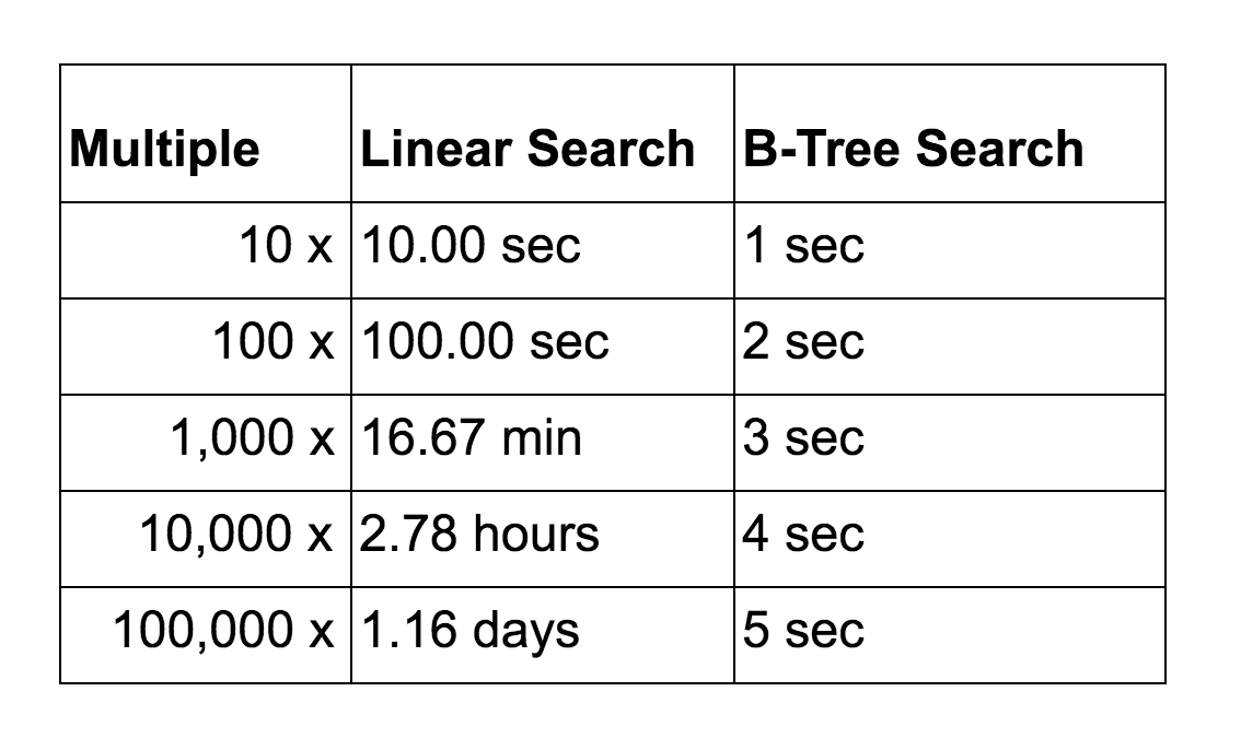
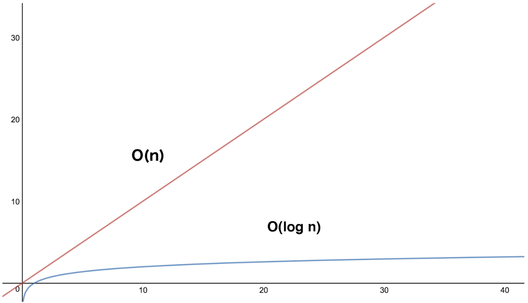
Below is a graph of the search time (y-axis) vs. the record count (x-axis). It is apparent that the B-Tree, which is the blue line, is more performant as the volume of records increase.
Indexes and Underlying Table Data Structure
Initially, SQL databases create indexes for each unique constraint and primary key by default.
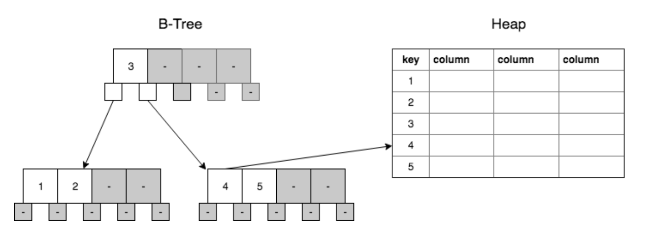
In a table with only non-clustered indexing, the underlying data structure of the table is a heap. This is quite efficient, as it is simple to add new records (or rows) to the database, as well as to the indexes (as long as the indexed values are unique and ever increasing). If the indexed column is not unique, and the values do not come in ever-increasing values, then the tree does need to be rebalanced at times, which requires more overhead.
In terms of implementation, the B-Tree has index values and associated pointers that point to the record in the aforementioned heap.
In the heap, each record has a pointer to the next record. Once a record in a heap structure is written, it does not move. Updating a value does not require a reallocation of disk space as long as the field is fixed width (majority of field types), meaning the space is preallocated for the largest value allowed in the field.
Additional Resources
A great one-stop-shop for increasing knowledge and comfort with SQL for developers can be found at Use The Index, Luke!. It is a phenomenal resource for dipping your toes into the SQL ocean.


